Brit Cruise

DEMO OF DYNAMIC INSTRUMENTATION:

Introduction

The purpose of this post is to propose a solution to the following future research directions offered in two papers on the Algorithmic Music Evolution Engine (AMEE) “A Flexible Music Composition Engine” and “Real-Time Emotional Adaptation in Automated Composition”, recently developed at UWO (Hoeberechts, Demopoulos, Katchabaw 2007)[10][11]. I’ve divided up the problems into two high level categories A and B:

A – Control theory for emotion

“We need to do more research to determine which emotions we want to be able to vary, and how those emotions will be translated into changes to musical elements … There is evidence that people only perceive certain emotions in music, but not others. Maybe we will find that some terms collapse into others”[10]

B – Expansion to the musical alterations made in the system

“Further literature research, refinements to existing emotions and possible extensions to other supported emotions and musical alterations…”[11]

“Presently, we do not change instrumentation based on emotion…Further thought and research is needed on this topic”[11]

“Informal feedback has indicated that some emotional changes are not as easily perceived in AMEE as others…”[11]

I will proceed as follows: First I will expand the conceptual model for how emotion should be modeled within AMEE. Then I will outline two avenues of expansions that could be made to low-level musical alterations in AMEE: Expressive Performance & Instrumentation/Sound synthesis. Each these topics will be broken down and explored in detail. I will conclude with directions for future research.

A: Conceptual Model of Emotion Control

AMEE’s initial prototype goal was stated as “dynamic music generation” it proceeded by first considering only musical score generation. This was an important focus as they developed a powerful, pipelined architecture for composition that is flexible, modular and extensible. This pipeline overseas the generation process of musical blocks as follows: The section producer is called on to get a new section of the piece, the block producer then returns a block (phrase), this is filled in with notes by the line producer and the completed block is sent to the output producer for synthesis. At each stage the emotionMapper class can make alterations adjustments to the music specified by the user.



[Figure 1 – AMEE’s pipelined architecture]

Since their target application is video game music, it is necessary that the system be capable of sound synthesis rather then musical score data only. Currently AMEE does this by sending the generated score, which is stored in MIDI format, to the default JAVA sound library for synthesis. However, this has resulted in some limitations. They mention that “some emotional changes are not as easily perceived as others” and they identify that future development is needed to both musicality and instrument quality. [11]. The main contribution of this thesis is to change the overall perspective of AMEE to address the root of these issues.

I propose that AMEE be viewed as an expert system for real-time orchestral composition and performance. This system is supposed to supplement the role of a real composer and orchestral performance. We must understand how an orchestra functions at all levels in order to correctly model an algorithmic approximation of one. Otherwise the system will be limited; for example, AMEE does not include instrument arrangement or the role of a conductor.

[Figure 2- The CPS approach to model mood control within an orchestra]

This would modularize AMEE into three independent subsystems, each of which is altered by the emotion mapper. I will refer to this as the CPS approach defined as follows (Figure 2):

Composition: The static elements one would find on a musical score within an orchestra (including global settings). This includes the musical notes, key signature, articulation marks, global tempo, time signature and volume.

Performance: The parameterized directions imparted by a conductor on a group of musicians. This involves the shaping of all audible performance parameters such as tempo, sound level, articulation, in order to contribute to the emotional communication of music [KTH]. In simple terms, this is the difference between a deadpan mechanical production of music and an expressive performance (See Apendix).

Synthesis: The instrument arrangement or equivalent electronic synthesis of sound to match the desired mood of the piece. In an orchestra the process of arrangement involves informed instrument choices for specific musical segments according to the mood. More specifically, this relates to all of the sonic aspects of sound unrelated to pitch and volume, commonly described as timbre.

AMEE currently considers C, a very primitive version of S and ignores P all together. In the following sections I will explore P and S in detail. I propose that even though C, P and S could be linked to a single mood, the system would be more powerful and flexible from a users perspective if they could adjust C, P and S independently.

This is a closely resembles how choices are made in a real orchestra: a composer creates a piece with some desired mood, an arranger interprets the score to match the emotional needs of the application (film or video game score, music therapy, live performance…etc.) and the conductor directs the individual musicians performance to fine tune the emotional expression of the work. If AMEE could adapt this CPS framework then it would offer the user a unique way to simulate all aspects of mood control. It would offer 3 degrees of freedom to find the correct mood for their specific application as opposed to the single degree of freedom currently offered. I feel it is important in an automated music system to decouple the creative decisions on this high level whenever possible – otherwise we are limiting the user.

A: Emotions in a Possibility Space

At the lowest level music composition and performance can be understood as making choices within multiple degrees of freedom. In this way, we can see that music is a time series of state transitions between multiple low-level features (or degrees of freedom). For example, in Western music we use a 12-tone scale that limits the possible note choices. In this domain (computer music) we are using MIDI standard representation [23] of music that consists of a series of event messages such as:

1. Pitch of a note (within 12 tone scale)

2. Intensity of the note (key pressure)

3. Note On event: This message is sent when a note is depressed.

4. Note Off event: This message is sent when a note is released.

5. Key Pressure: This defines the volume at which a note is played

6. Instrument Mapping

When a musician performs or composes a piece of music to match some desired emotional quality, they will adjust the above features. For example, they may play slower or increase articulation (Articulation = Note On event – Note Off event). Emotions are viewed as complex psychological constructs, although, when encoded into MIDI data some common patterns emerge. Recall we are not trying to define emotion, but rather define links between emotional descriptors and primitive aspects of low-level musical representation. In this way we can view emotions as well defined regions within a possibility space. Or more precisely, every possibility space can be colored according to dominant emotional affect within some region.

AMEE’s emotionMapper (defined in following section) controls the following elements: tempo, dynamics, articulation, mode, tonal consonance and pitch. This defines the 6-dimensional space that AMEE alters in order to communicate emotions.

This idea of space coloring is equivalent to the task of high-level musical classification algorithms. In this case the task is precisely the reverse of AMEE: To categorize raw music signals into abstract categories such as genre, style or mood. This is based on the proven theory that meaning in music is communicated through alterations to low level features; the goal is to find the most salient features [7]. The concept of musical classification has been around for decades and is still an active research area. The general training procedure is as follows:

1. Input a musical signal (which are selected according to mood, genre, style…)
2. Extract salient low-level features (such as tempo, timbre, meter, dynamics…)
3. Based on the values of these features learn to classify a musical signal into categories using multidimensional scaling.

Using a classification procedure to learn rules is a logical approach to develop expert systems. Although well known musical rules exist, classification algorithms provide us with more detailed data that would not otherwise be known. I present this here to inform the following discussions on emotion control and low-level features.

A: Strategy for Emotion Control

AMEE’s Approach

This section presents a comparison between AMEE’s current strategy for mood control and an optional dimensional approach. In AMEE, the class through which the user controls emotion is called the emotionMapper. It is linked to the dimensionAdjustment class that performs the necessary calculations. It works as follows; the user can adjust 10 emotional variables from 0 (emotion not present) to 100 (emotion present). The emotions they chose to include are: Happy, Sad, Triumphant, Defeated, Excited, Serene, Scared, Ominous, Angry and Crazy. Every emotional variable is then linked to each of the six dimensions (tempo, mode, dynamic, articulation, consonance, pitch). A number (contribution) between -1.0 and +1.0 defines the polarity and strength of influence each emotion has on the musical characteristic. Because multiple emotions can be adjusted (intensity), at the same time, the dimensionAdjustment class combines the effect all adjustments made on each dimension as follows:

It is this combined calculation of emotion contribution that defines how the system models the current mood. The choices for how each emotion influenced every dimension was decided heuristically by comparing results from a variety of other studies, the more prevalent the effect (such as serene = +1.0 consonance) the closer the value is to +1.0. This method is based on the following logic: If we allowed the user to control each of the 6 dimensions independently, it would be very difficult if not impossible to change between emotions easily. Instead, the user controls one emotion variable that is linked to a parallel adjustment of 6 low-level features. The emotional intelligence in this system is entirely contained within the dimensionAdjustment class as it defines how these parallel adjustments are made. This is also the key element to one of the system’s patent This strategy is novel, although, it leads to the following issues:

Issue 1 – If new low-level elements (dimensions) are included in the system, then each dimension must be independently linked to every emotion slider. If the low-level element is difficult to understand at a high level, (such as spectral similarity or timing deviations) then this process becomes time consuming and imprecise. This same logic applies if we were to include a set of new emotion variables.

Issue 2 – This process cannot be automated since it’s up to the programmer to define how each emotional variable is linked to new dimensions. This can lead to inconsistencies and result in an unclear picture of how the system models emotion. If we were to include 10 new low-level attributes (as described in the following section) then 10 different programmers would give 10 different answers.

To visualize AMEE’s emotion control in terms of a possibility space, I constructed the following plots using data directly from the dimensionAdjustment class:

[FIGURE 3: Left – Expressive dimensions Right – Composition dimensions]

I divided the six dimensions into two plots. On the left is a plot using the three dimensions related to expression, as they have no effect on which notes are played. On the right is a plot using the three dimensions related to composition as they effect notes played. Each axis contains the dimension’s contributions with values from -1.0 to +1.0. Each vector in the graph represents a single emotion variable (at full magnitude) as follows:

EMOTION	COLOR
happy	Red
sad	blue
triumphant	orange
defeated	green
excited	Black
serene	light blue
scared	purple
angry	yellow
ominous	light green

These plots clarify how adjusting an emotion variable is equivalent to extending along the corresponding emotion vector. A neutral setting would exist as a point in the center of both graphs, as we increase happiness, the points would travel along the red vector. Notice how emotions that are well-defined opposites have inverse directions in both graphs (such as happy-sad and serene-angry).                   

Proposed Dimensional Model of Emotion

It is challenging to assign unique meanings to each emotional state; a dimensional approach allows us to strategically decompose them into the underlying components. This view is well defined in a 1954 article by Schlosberg titled “Three Dimensions of Emotion” [20]. The two primary dimensions were one of affective valence (ranging from unpleasant to pleasant) and one of arousal (ranging from calm to highly aroused). A third dimension was called dominance or control which the submissiveness or dominance of an emotion (angry is more dominant, scared is more submissive). Dimensional views of emotion have been advocated by a large number of theorists through the years, including Wundt (1898), Russell (1974), and Tellegen (1985) [8]. The most famous model of emotion in the English language is the Circumplex Model of Affect proposed by Russell in 1980 [1]. This is a spatial model based on the two primary dimensions of affect and valence. Affective concepts (emotions) fall into 2D space according to their relation to valence arousal. From now on, I will refer to this as the VA space model. Figure 4 shows this model of valance and arousal along the horizontal and vertical axis respectively.

[Figure 4: Russell’s Circumplex Model of Affect [12]]

This model of emotion is extremely useful for music composition systems as it eliminates ambiguity and provides a consistent global model of emotion. Notice how the paired emotions happy-sad and serene-angry (identified earlier) also appear on opposite sides of this map. This VA model has been adopted in different ways by a large body of research related to emotion control and algorithmic composition systems related to performance, composition and synthesis [3][15][4]. These systems use the VA map as a control strategy and present the user with a 2D plane to define the affect quality of the system [7].

I propose that embedding a VA space within the emotion mapping process can solve both control issues I defined in AMEE’s control strategy. The following is a new framework for emotional control:

1. User inputs emotion intensity levels using the existing variable sliders. In this case we would only use well defined emotions from the VA plot and eliminate variables such as crazy and scared since they are not well defined in VA space.

1. Each emotion is represented as a vector in VA space. The direction of the vector is defined according to the placement of each emotion in the Circumplex model. Figure 5 shows the 7 emotions AMEE is using which are well defined within the VA space according to the color mapping in Figure 4.

[Figure 5: Vector plot of emotion inside VA space]

1. Every low-level dimension’s contribution is mapped independently to this VA space. This is modeled as a three-dimensional surface as in Figure 6. The third dimension (k) represents the contribution from -1.0 to +1.0. Here the k represents the contribution of a single dimension such as consonance, volume, tempo…etc.

[Figure 6: Mapping a low level element (k) over VA space. [7]]

This surface can be defined in different ways depending on the musical element in question. If a low-level element had no contribution to any emotion then it would exist as a flat surface. Or, if a low-level element, such a volume, is correlated with arousal only the plane would be modeled as Z = A in Figure 6.

[Figure 7: possible tempo mapping vs. neutral mapping]

The equation, which defined this k-plane (contribution), can come from well-known musical rules of thumb, existing research, or data learned from classification algorithms. This method is powerful since non-linear relationships can also be defined by shaping the surface accordingly. See the chapter on timber for a deeper explanation of this.  Linear mappings between VA and musical features has been adopted by Fridberg and more complex contour mappings are defined by Wu [7][21].

1. Combine the effect of each emotional by performing vector addition within VA space. Figure shows the result of combining happy and serene at full intensity.

[Figure 8: Vector addition in VA space]

1. The resultant point from 4 in the VA space will be mapped independently to each low-level dimension according to the plane defined in 3. This will result in a vector of adjustments that are made on all low level elements. This is exactly the same vector which is calculated in AMEE’s current dimensionAdjustment class

This strategy is powerful since we can now include any number of low-level musical dimensions linked to any number of emotional variables by defining the equation of a single plane or surface. This avoids inconstancies, increases flexibility and expansion, and defines a clear global perspective of emotion.

B: Expansion to the Musical Alterations

Expressive Performance

In music, expressive performance can be controlled by an individual performer’s motive, or in the case of an orchestra, by the conductor. This is done through gestures that mediate and control the subtle changes to the volume, speed, and articulation of a performance. These have been shown to be the three most important parameters used to communicate emotion in music [8]. Even in the case of solo neutral performance, a human will impart some small natural, or random, deviations to the score. If the same solo performer intends to express some level of arousal/valence into their performance the deviations may grow and shrink accordingly (mp3 audio example follows in Appendix A). Recall the goal is not to define global attributes of volume, speed and articulation, but to define how they deviate from a global value over time. The magnitude and direction of these deviations must then be linked to VA space. Although this may seem overly subjective, it has been shown that common performance standards exist for different performers of varying skill levels [8]. Encoding these general patterns into a VA space would provide the power to control the expressive quality of generated music according to specified mood.

Canazza, Roda, Zanon, Friberg developed the expressive director system which allows real-time control of music performance synthesis. It allows the user to change the expressive style in real time according to emotional intent. Their system merges the KTH rules [6] and the CSC system[3]. It works over a valence arousal space and is modeled within the MIDI framework, making it an ideal candidate to guide implementation within my proposed VA embedded control scheme. The KTH rule system is a set of 30 rules that musicians use to transform a score into a musical performance. The list is extensive so I’ve extracted some key rules which related to the features I propose:

1) Phrase arch: Create arch-like tempo and sound level changes over phrases

2) High loud: Increase sound level in proportion to pitch height

3) Duration contrast: Shorten relatively short notes and lengthen relatively long notes

4) Faster uphill: Increase tempo in rising pitch sequences

5) Double duration: Decrease duration ratio for two notes with a nominal value of 2:1

6) Punctuation: Find short melodic fragments and mark them with a final micropause

7) Score legato/staccato: Articulate legato/staccato when marked in the score

8) Repetition articulation: Add articulation for repeated notes.

The CSC system is a model based on the hypothesis that different expressive intentions can be obtained by suitable modification of a neutral performance. They represent this as a expansion/compression (exaggeration/attenuation) of three low-level parameters (which they define as sonologic parameters): S^MM (tempo), S^KV(volume), S^LEG(articulation). The value of tempo, volume and articulation depends at any moment on the score value of the current note n (or global setting) and the expressive deviation calculated as:

S^k (n)= global shift + k*P(n)                                                                                                 (1)

In this case k is the control parameter that adjusts the amount of deviation applied to the global level and n is the current note. P^k is the expressive profile, of parameter k, calculated over a sliding window as:

P^k(n) = S(n) – S_avg(n)                                                                                                             (2)

Here S_avg is the expressive profile of the parameter average centered on the nth note. S(n) is the value of a neutral performance. The following explains how this system could be implemented into AMEE starting from step 3 of my control procedure:

3) Three new low-level parameters must be included in the system: k_t, k_d and k_a. Each of these can be defined as a flat surface (linear relationship) on the VA space calculated as:

k_i(x,y) = neutral setting + x*(valance weight) + y*(arousal weight)                                 (3)

These valance and arousal weights come out of multi-dimensional analysis of perceptual tests [3].

4) Once user makes an emotion adjustment, the combined mood setting is expressed as a coordinate in VA space (x,y) as previously defined.

5) From this coordinate we can calculate each low-level parameter k_t, k_d and k_a

using (3). From these k values we can calculate the expressive profiles for tempo, volume and articulation with (2). Finally each parameter S^k is calculated as in (1).

It is convenient that this method controls the exact same expressive variables I have grouped together in the previous plots demonstrating possibility spaces for emotion. We can now to clarify the difference between a mechanical performance and an expressive one in terms of this space.

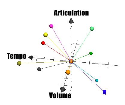
Figure 9 shows the difference between a static happy setting for tempo, volume and articulation (right) and an expressive setting (left). The sphere defines the expression/expansion of each dimension (tempo, articulation, volume); the radius of the sphere represents the amount of deviation (expression/expansion).

[Figure 9: Expressive vs. Mechanical performance within TempoVolumeArticulation space]

Timbre

The task is to control the timbre of a sound to have some desired emotional qualities. This requires an understanding of the relationship between low-level audio features and more abstract terms (such as valence and arousal). Audio classification algorithms based on timbre have the opposite goal: input a raw signal and extract spectral features and classify into high-level classes (such as genre, or style). Analyzing high-level feature extractors we can look for general patterns in the way features can be constructed from the bottom up. The first goal is to identify what low level musical features are relevant and how they are represented.

[Figure 10: tempo extractor and the low level operations involved [18]]

The analysis and alteration of audio signals is described as Audio Signal Processing. First, audio needs to be defined as a time to amplitude function (or pressure wave). Digital audio is a stream of numbers that represent the amplitude of a signal at each point in time (number of points in time is called the sample rate, the number of values each measurement can take is called the sample resolution). Audio processing functions can be represented in an analog or digital format. Analog processing directly alters the electrical signal (a volume knob controls a variable resistor or potentiometer) while digital processing (DSP) performs mathematical operations on the binary representation of the signal (Volume is changed by multiplying each sound sample by some value). To proceed we must understand that DSP is operating on the following three dimensions: time, frequency and amplitude.

Timbre defines the quality or color of a sound; every sound producing mechanism has a unique spectral and temporal fingerprint. Voices or instruments of different timbre will sound distinct from each other even if they are producing the same pitch at the same amplitude. The spectrum of a sound is a frequency amplitude function, as every sound is comprised of a collection of frequencies at different energy levels that vary over time. Spectrogram analysis of this function allows unambiguous quantification of these energy levels at each frequency over time.

[Figure 11: A spectrograph analysis of a sound]

The spectral envelope is captured along the vertical axis of the graph, while the temporal envelope is described along the horizontal axis of time in Figure 11. Temporal envelope is comprised of the following four features: attack, decay, sustain and release defined as:

Attack time – The time taken for initial run-up of level from nil to peak.

Decay time – The time taken for the subsequent run down from the attack level to the designated sustain level.

Sustain level – The amplitude of the sound during the main sequence of its duration.

Release time – The time taken for the sound to decay from the sustain level to zero after the key is released.

Next we must understand how relevant patterns can be extracted from this fingerprint for both classification and synthesis.

Musical features related to Timbre

The type and number of musical features that can be extracted from a sound signal are immense; however, some features are more commonly used in music classification tasks. These features should therefore be relevant when defining the direction of synthesis into predefined categories. The work done by Tien-Lin Wu and Shyh-Kang Jeng is useful as they propose a novel method to automatically classify the emotions of musical segments (using 10 second sliding windows) [21]. They use a Support Vector Machine to classify 75 musical segments into the 4 quadrants (4-class classification) of the VA space. To do so 55 different features are extracted from a musical segment, which are reduced with feature selection methods that determine the ones with best classification performance.

They compared different feature subsets and achieved accuracy of 98.67% (leave-one-out cross-validation) emotion classification. The 55 features used in their study can be broken down into the following sets: Rhythm, Dynamics, Pitch, Timbre and Space. They also note some interesting relationships between each emotion class (quadrant) and the musical features by comparing with musicians rules of thumb. Of the 21 features in the timbre set the most relevant for classification was frequency centroid (FC), commonly described as the brightness/dullness of a sound. FC measures the average frequency weighted by amplitude of a spectrum. We can calculate the individual centroid for each frame on a spectrogram as follows:

Where c_j is the average frequency weighted by amplitudes, divided by the sum of the amplitudes. The following plot shows both the musician rule of thumb for timbre as well as the contour plot of the FC classification data (Figure 12).

[Figure 12: Musicans’ rule of thumb, Right: Contour plot of  data[4] ]

As a rule, brightness is related to large arousal and positive valence. The FC data shows a correlation between FC and higher arousal, which is consistent. Another important feature to include which captures the rule of thumb for harshness is spectral dissonance (SD) [4]. SD describes the smooth/harshness or stability of a sound. It is important to clarify this can be understood at the note level and spectral level. Note intervals will have certain consonances and AMEE models this aspect already (by shifting by a half tone). At the note level a highly consonant interval would be a perfect fifth or octave pair, a dissonant interval would be a minor second or major seventh. At the spectral level consonance is defined by existence of harmonics (or overtones) that are pleasing to the ear. The physical definition of this is a wave whose frequency is a whole-number multiple of another (the so called fundamental frequency). In AMEE we can use this information when making decisions for both tonal consonance (harsh tone interval or chord) and spectral consonance (harsh sounding instrument).

A useful experiment done by Plomp and Levelt examined how listeners perceive consonance [19]. They generated pairs of sine waves and had volunteers rate them in terms of their consonance. A trend emerged which is shown in Figure 13. When two tones are produced as almost the same frequency there is a beating effect people perceive due to the interference between the two tones, this beating disappears when the two tones are at identical frequencies.

[Figure 13 : Dissonance vs Frequency Ratio [19] ]

Figure 19 shows how dissonance varies according to intervals, notice how perfect fifth and octave intervals are more consonant than a minor second. This information can also help us expand the ability of AMEE to model tonal dissonance.

Wu and Jeng also present the following plot relating spectral dissonance (harmony) to VA quadrants for both rules of thumb and classification data. Their experimental results show that strong dissonance is associated with high arousal and low valance levels.

[Figure 14: Musicans’ rule of thumb, Right: Contour plot of SD data[4] ]

To identify other useful features I also explored the work of Olivera and Cardoso in their paper titled “Emotionally-controlled Music Synthesis” [16]. This paper was a background study done to support their work on a system that produces music with appropriate affective content. I also explored the following summary of their system, which they published in 2009 [17]

Along with frequency centroid and spectral dissonance they also identify the following spectral features and their relationship to the VA space: spectral flatness and timbral width. To understand these we must first define specific loudness: The parts of the frequency spectrum that make the strongest contribution to loudness [2]. Timbral width is a measure first proposed by Malloch [13], it measures the flatness of the specific loudness function. Spectral flatness (or sharpness) is similar except it is calculated by dividing the geometric mean of the power spectrum by the arithmetic mean as follows:

x(n) represents the magnitude (or power) of the frequency “bin” n, where N is the number of frequency bins used in the calculation. An example of a spectral flatness would be white noise since it is defined as having equal power in all spectral bands. As expected timbral width and spectral sharpness have similar locations in the VA space since they are functionally similar.

These are the correlation coefficients found by Olivera and Cardoso between these features and valence/arousal using regression models:

Spectral Sharpness    Valence: 0% Arousal: 44%

Timbral Width           Valence: 0% Arousal: 54%

The final feature AMEE should incorporate are independent concepts of loudness and volume. Currently AMEE models volume as it relates to amplitude and sound pressure. It does not include loudness as a low level feature. Loudness is more subjective a measure influenced by the frequency spectrum and bandwidth. A simple example would be the difference between a single instrument producing a musical line and multiple instruments producing the same musical line. This may not increase the decibel level of the sound but a listener will describe it as sounding fuller or bigger. I will leave the application of this low level feature for future work.

This research resulted in the following list of spectral features that are strongly correlated to valence and/or arousal. I have combined correlation coefficients are a combined result from Olivera, Cardoso, Wu and Jeng’s studies:

Frequency Centroid     Valence: 20%   Arousal: 80%

Spectral Dissonance    Valence: 28%  Arousal: 72%

Timbral Width             Valence: 0%    Arousal: 54%

Spectral Sharpness     Valence: 0%    Arousal: 44%

With the relevant low-level timbral elements we proceed in two ways: Affective Instrumentation and Sound Synthesis:

Affective Instrumentation

This process is the orchestral equivalent of the arrangers’ task: to assign instruments according to the desired mood of the piece. This process is unambiguous and proceeds as follows:

1. Build a sound bank of instruments or acquire an existing one
2. Analyze every instrument according to each spectral characteristic
3. Plot the location of each instrument within an appropriate region of VA space

In order to prove the effectiveness of dynamic instrumentation within AMEE, I constructed a much simpler proof of concept as follows:

1. Analyzed the default sound bank provided by JAVA which AMEE currently uses
2. Link emotional sliders to three phases of instrument thresholds
3. Transition between instruments @ 0.2 , 0.5 and 0.7 slider intensity values

I choose to use the emotional sliders linked to “serene” and “ominous” to test out this process. I found it was helpful to choose emotions that exist on opposite sides of the VA space to simplify the calculation and demonstrate a wider sonic range. I also used this rough collection of instrument mappings to help inform my choices:

High Valence – Piano, Strings, instruments with few harmonics (flute or synthesized

sounds), bright trumpet.

Low Valence – Brass, low register instruments, string ensembles, violin, woodwind and piccolo.

High Arousal – Brass, bright trumpet, timpani.

Low Arousal – Woodwind, classic guitar, lute and soft sounding instruments.

I used the same technique AMEE implements in their dimension adjustment class, to link both emotion levels to instrument choices.  Now, when the user makes a change to the emotion slider, the following calculation is performed:

Instrument Choice = (Triumphant Level) – (Defeated Level)

This instrument choice variable is then placed into one of 6 bins depending on its value (which ranged from -1.0 to 1.0). From my initial listening tests and feedback from volunteers, it is apparent that this effect greatly enhances the emotional changes perceived in AMEE. This directly addressed the proposed “improvements to musicality” as defined in the AMEE literature. What is interesting about this method is that it allows an infinite variety of possible instruments with a simple extension. Instead of mapping one instrument to each region of the VA space, we can map a collection of instruments. This would allow the user, or the system, to cycle through different options within some static mood setting. This could be implemented as a pseudorandom choice, or it could be user controlled. The proof of concept code was inserted into standardLineProducer class within the fillMusicalBlock() method (see Appendix B).

Sound Synthesis

The research into spectral features and valence arousal also leads us to a more powerful potential option for future research. Using a real-time audio synthesis environment, we can “build” sounds through processes, such as additive or subtractive synthesis to achieve some desired spectral characteristics. I used the Super Collider audio synthesis environment for testing out some primitive aspects of these methods. I will briefly summarize below using SC source code to demonstrate:

Subtractive Synthesis

Subtractive Synthesis is a sound production process that starts with a complex audio signal and then removes harmonics one step at a time. This is done with the application of different audio filters to sculpt the sound into a desired quality. The initial source can be anything from noise (SC provides white or pink noise generators) to oscillators producing saw tooth waveforms. SC provides many filters, for example low/high/band pass filters which attenuate energies above and/or below a threshold. If we wanted to simulate the sound of a bowed string instrument we could proceed as follows:

1. Start by generating a saw tooth oscillator:

{ LFSaw.ar(500, 1, 0.1) }.play   // Frequency is 500hz, initial phase offset is 1, multiplier = 0.1

1. Apply a low pass filter to this source signal by plugging them into each other:

LPF(LFSaw.ar(500, 1, 0.1), 450) // LPF(source signal = saw tooth, cutoff frequency = 450HZ)

By tuning these parameters, we can find a natural approximation of the sound produced by a bowed instrument. The power with this low-level approach is that we can alter an instrument to have some desired spectral qualities. We could begin with a soft string instrument and slowly transition into a harsh one by adjusting appropriate parameters.

Additive Synthesis

Additive Synthesis is a process that begins with simple building blocks (such as sine waves), which are added together to form a desired sound spectrum. Any complex tone “…can be described as a combination of many simple periodic waves or partials, each with its own frequency of vibration, amplitude, and phase.”[22] To proceed in this way we must understand each instrument as a recipe for some spectrum. For example the following is a spectral recipe for a minor third bell:

500*[0.5,1,1.18,1.56,2,2.51,2.66,3.01,4.1]

Here the bass frequency is 500HZ and the inside numbers are the harmonic partials. So in order to generate this sound we must apply a sine wave generator to each partial:

{Mix(SinOsc.ar(500*[0.5,1,1.18,1.56,2,2.51,2.66,3.09,4.1],0,0.1))}.play

In this case each harmonic partial would be generated with the same volume, although this can be easily extended to include an array of independent volumes:

{Mix(SinOsc.ar(500*[0.5,1,1.18,1.56,2,2.51,2.66,3.09,4.1],0,0.1*[0.25,1,0.8,0.4,0.9,0.4,0.2,0.6,0.1]))}.play

This is only an introduction to the numerous possible sound synthesis methods. What is important to realize is that key parameters within these SC expressions can be easily linked to variables. These variables can then by mapped according to a VA space or emotional slider. The research I’ve done into spectral features will help mediate the choices made in terms of what parameters to adjust and how to adjust them. In order to demo this flexibility one can use the mouse coordinates to adjust the parameters in real time as the following example expression shows. Notice that the 1^st and 2^nd harmonic partials are now calculated dynamically according to mouse coordinates:

{Mix(SinOsc.ar(500*[ MouseX.kr, MouseY.kr)],,1.18,1.56,2,2.51,2.66,3.09,4.1],0,0.1*[0.25,1,0.8,0.4,0.9,0.4,0.2,0.6,0.1]))}.play

Conclusion

The following work presented a new control strategy to improve AMEE’s ability to model emotions. It resulted with a proposed change to the overall structure of emotion control – which I’ve named the CPS approach. To support this change a new freamwork for emotion control was also defined. This lead in two new modules for the system to adopt: Expressive Performance and Instrument Synthesis. Each of these modules was defined and relevant research used to identify the most salient low-level features required to model emotional affect. All of the initial questions outlined in the introduction of this report (broken down into A and B) have been addressed and solutions proposed.

Future Work

1. Implement the new CPS control strategy in AMEE.

1. Write a synthesis and expressive performance module based on the research done and incorporate the new low-level elements defined in this report.

1. Explore how different expressive profiles could be stored in pattern libraries by users.

1. Explore generative music models as an optional method to encode expressive performances (and improve melody generation). This topic has been explored, but not relevant to this report specifically, an initial outline is listed in Appendix C.

1. Improve the simplified linear model of expressive performance outlined and incorporate more of the KTH rules.

References

1) Altarriba, J., Basnight, D. M., & Canary, T. M. (2003). Emotion representation and perception across cultures. In W. J. Lonner, D. L. Dinnel, S. A. Hayes, & D. N. Sattler (Eds.), Online Readings in Psychology and Culture (Unit 4, Chapter 5), (http://www.wwu.edu/~culture), Center for Cross-Cultural Research, Western Washington University, Bellingham, Washington USA

2) Cabrera, D. “Psysound: A computer program for psychoacoustical analysis tripod.com.” Proceedings of the Australian Acoustical Society Conference, Melbourne. 24.26 (1999): pg. 47-54

3) Canazza, Sergio, Antonio Roda, and Patrick Zanon. “Expressive Director: A System For The Real-Time Control Of Music Performance Synthesis.” Proceedings of the Stockholm Music Acoustics Conference. (2003): pg 1-4.

4) D’Inca, Gianluca, and Luca Mion. “Expressive Audio Synthesis: From Performances To

Sounds.” Proceedings of the 12th INternational Conference on Auditory Display. (2006): pg 2-3.

5) Eck, D. Measuring & Modeling Musical Expression: NIPS 2007 MBC Workshop Expressive

performance dynamics. 2007 pg.5-12

6) Friberg, Anders, and Roberto Bresin. “Overview of the KTH rule system for musical .”

Advances in Cognitive Psychology. 2.2-3 (2008): pg 145-161.

7) Friberg, A. “pDM: An Expressive Sequencer with Real-Time Control of the KTH Music- Performance Rules.” Computer Music Journal, MIT Press. (2006): pg 2-5.

8) Grindlay, Graham, and David Helmbold. “Modeling analyzing, and synthesizing expressive piano performance with graphical models.” Machine Learn. 65. (2006): pg 361-387.

9) Huron, David. Sweet Anticipation – music and the psychology of expectation.

Cambridge: MIT Press, 2007.

10) Hoeberechts,  Demopoulos, and Katchabaw.  A Flexible Music Composition

Engine.  Proceedings of AudioMostly 2007:  The Second Conference on Interaction with Sound.  Ilmenau, Germany, September 2007.

11) Hoeberechts, Shantz. Real-Time Emotional Adaptation in Automated Composition. Proceedings of Audio Mostly 2009: The fourth Conference on Interaction with Sound.  2009.

12) Lang, P.J., Bradley, M.M., & Cuthbert, B.N. Technical Manual and Affective Ratings. NIMH Center for the Study of Emotion and Attention . 1997. Print.

13) Malloch, S. “Timbre and Technology: An Analytical Partnership.” Contemporary Music Review. 19.2 (2004): pg 53-79.

14) Meyer, L. B. Emotion and Meaning in Music. The University of Chicago, 1956.

15) Oliveira, Antonio, and Cardoso . “Towards Affective-Psychophysiological Foundations for Music Production”. Lecture Notes in Computer Science. (2007): pg 2-4.

16) Oliveira Antonio and Amilcar Cardoso. “Automatic Manipulation of Music to Express Desired Emotions.” Proceedings of the AMC 2009 – 6th Sound and Music Computer Conference, Porto – Portugal, 23.25 July 2009. pg 2-5

17) Oliveira Antonio and Amilcar Cardoso, “Emotionally Controlled Music Synthesis”, 10th regional conference of AES Portugal, Lisboa, 13 – 14 Dec. 2008.

18) Pachet , F, and P Roy . “Analytical Features: A Knowledge-Based Approach to Audio Feature Generation .” EURASIP Journal on Audio, Speech, and Music Processing . 2009.Article ID 153017 (2009): pg 3-13

19) Plomp , R, and WJM Levelt. “Tonal consonance and critical bandwidth.” journal of the Acoustical Society of America. 38.4 (1965): pg 548-560

20) Schlosberg, H. “Three dimensions of emotion.” Psychological review. (1954): Print.

21) Wu, TL, and SK Jeng. “Automatic emotion classification of musical segments.” 9th International Conference on Music Perception and Cognition (2006): n. pag. Web. 30 Mar 2010.

22) Thompson, W. Music, Thought, and Feeling: Understanding the Psychology of Music. Oxford: Oxford University Press, 2008. pg 46.

23) Unknown Author. “Table 1 – Summary of MIDI Messages .” MIDI Manufacturers Association. N.p., 20/03/2010. Web. 30 Mar 2010. http://www.midi.org/techspecs/midimessages.php

This entry was posted on May 31, 2010 at 4:59 am and is filed under Random Stuff, Research and Projects with tags "Computer Music", additive synthesis, algorithmic music composition, algorithmic music for video games, Algorithmic music synthesis, Amilcar Cardoso, Antonio Oliveira, aritifical orchestra, Artificial Intelligence, circumplex model of emotion, computer science, dimensions of emotion, douglas cope, Douglas Eck, emily howell, emotion control in generative models, Expressive performance algorithms, generative models of music, Generative Music, low-level music features, mood control, music affect, music and emotions, music and mood, music classification, sprecturm, subtractive synthesis, timbre, video game music. You can follow any responses to this entry through the RSS 2.0 feed. You can leave a response, or trackback from your own site.